Fast and automatic tuning and fitting for group lasso penalized least squares

Fits group lasso penalized least squares model over regulraization path determined by intermediate estimates of noise variance \(\hat \sigma^2\).

Usage

autotunegg(
  x,
  y,
  group,
  alpha = 0.01,
  standardize = TRUE,
  standardize_response = TRUE,
  intercept = TRUE,
  active = NULL,
  trace_it = FALSE,
  sigma_tolerance = 1e-08,
  beta_tolerance = 1e-08,
  sigma_iter_max = 100,
  beta_iter_max = 100,
  active_iter_max = 100,
  tau = 0.5
)

Arguments

x

Matrix of predictors, of dimension \(n \times p\) with \(n\). observations of \(p\) variables

y

Vector of responses, length \(n\).

group

Vector of consecutive integer group labels, length \(p\)

alpha

Significance level for sequential Wald tests, default is 0.01

standardize

Whether to standardize prior to tuning and fitting, default is TRUE. Coefficients are transformed back to original scale after model convergence. Strongly recommended as this algorithm does not implement standardized group lasso.

standardize_response

Whether Y is demeaned, default is TRUE.

intercept

Whether to include an intercept, default is TRUE.

active

Whether to implement active set selection. Default is TRUE when all groups have 5 or more members, and FALSE otherwise.

trace_it

Whether to print out iteration details, default is FALSE.

sigma_tolerance

Convergence termination tolerance for the initial tuning of \(\sigma^2\) and \(\lambda\). Default is \(1e-8\).

beta_tolerance

Convergence termination tolerance after \(\sigma^2\) and \(\lambda\) are obtained. Default is \(1e-8\).

sigma_iter_max

Maximum number of iterations allowed for the initial tuning of \(\sigma^2\) and \(\lambda\). Default is 100.

beta_iter_max

Maximum number of iterations allowed after \(\sigma^2\) and \(\lambda\) are obtained. Default is 100.

active_iter_max

If active = TRUE, limits the number of updates to the active support set. Default is 100.

tau

Scaling for initialization of \(\lambda\). Initial \(\lambda = \lambda_{\max} \times \tau\). Must be smaller than 1 or the algorithm will get stuck. This scaling is removed once \(\hat{\sigma}^2\) is smaller than \(\text{Var}(Y)\).

Value

A list with final model fit as well as regularization path details.

Examples

# generate simple data
library(autotunegg)
set.seed(2026)
n <- 100
pg <- 10
p <- pg*n
group <- rep(1:n, each = pg)
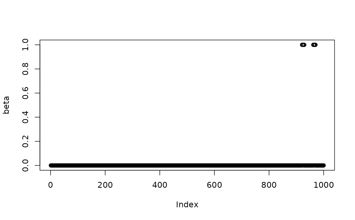
# 2 target groups (beta = 1)
s <- 2*pg
beta <- rep(0,p)
beta[group == sample(unique(group), 2)] = 1
x <- matrix(rnorm(n*p),n,p)
snr <- 4
error.sd <- sqrt(sum(beta^2)/ snr)
err <- rnorm(n, 0, error.sd)
y <- x %*% beta + err
fit <- autotunegg(x, y, group, active = TRUE, trace_it = TRUE)
#> 
Iteration: 1
Iteration: 2
#> No of predictor group significant for sigma estimation: 2
# # plot beta's
plot(beta, pch = 1)

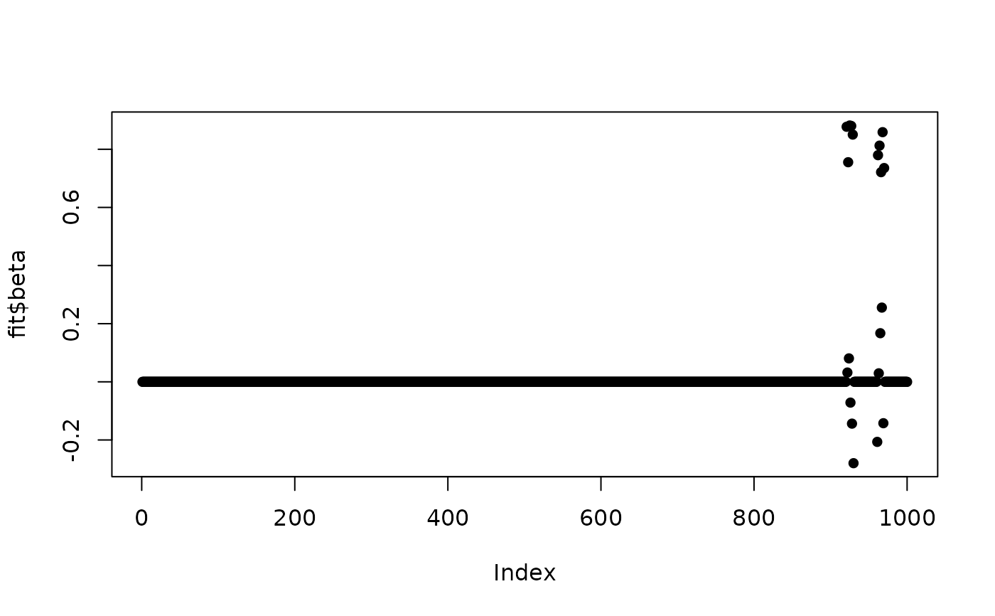
plot(fit$beta, pch = 16)

# print confusion matrix
table(beta == 1, fit$beta == 1)
#>        
#>         FALSE
#>   FALSE   990
#>   TRUE     10
# Estimated \eqn{\hat \sigma^2} path vs empirical
fit$CD.path.details$count_sig_beta
#> NULL
var(err)
#> [1] 2.485548