Getting Started with prolong

library(prolong)

The prolong package has two primary objectives:

Facilitate the penalized modeling of high-dimensional longitudinal omics data with a longitudinal clinical outcome to obtain a sparse set of omics variables that co-vary with the outcome over time
Provide functionality in both R and in a point-and-click GUI shiny app for plots that reveal the underlying dependence structure of the omics variables

For the first objective, the prolong() function takes an \(n \times t\) matrix of clinical outcomes and a \(n \times p \times t\) array of omics or omics-like variables and fits a model with a network penalty via laplacian matrix together with either a lasso or group lassa penalty. Hyperparameters can either be supplied or automatically estimated internally in prolong(). The plot_trajectories() function takes the output from prolong() and displays a grid of the trajectories of the variables selected by the (group) lasso + laplacian model.

For the second objective, the prolong package will eventually sypport several plot functions that take the same \(n \times p \times t\) array of omics or omics-like variables and look at the pairwise correlations of the first-differenced, or delta-scale, omics or omics-like data. The following function is currently supported:

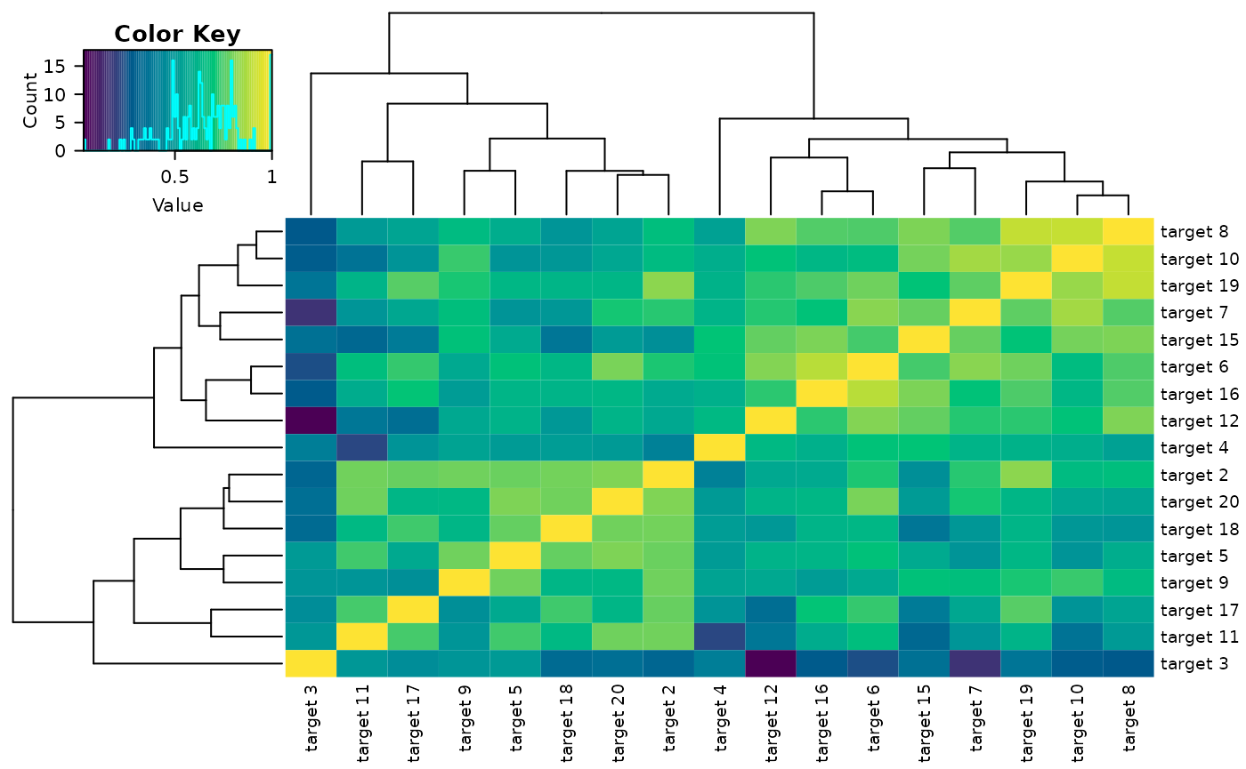
delta_heatmap() - Interactive subsettable heatmaps

The prolong package comes with example data that is simulated to imitate the motivating data for the prolong methodology. There are two components that can be accessed with the load() function:

sim_metabs Simulated variables in a \(15 \times 100 \times 4\) array
sim_outcome Simulated outcome in a \(15 \times 4\) matrix

Example Data

The prolong package comes with example metabolite-inspired variables and viral load-inspired outcome simulated to imitate the real data that motivated prolong.

Example Outcome

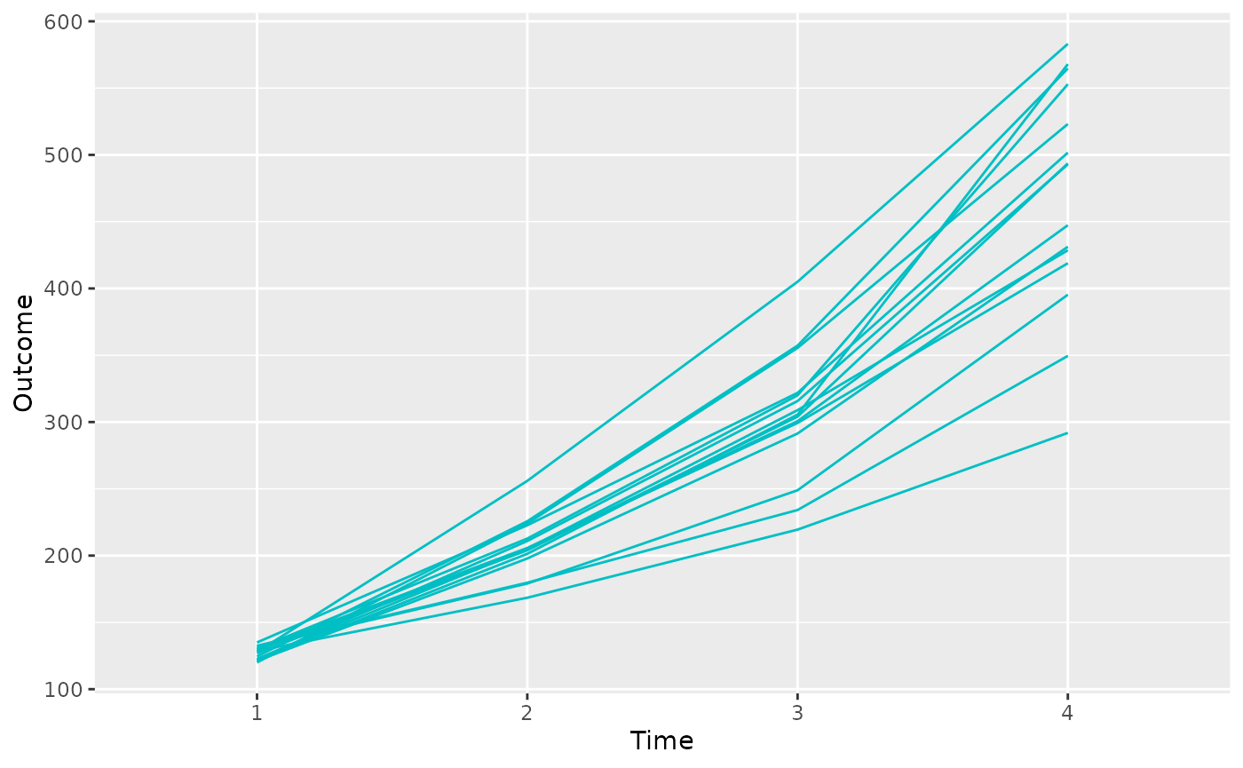
The example outcome data can be accessed with:

data("sim_outcome")

This simulated clinical outcome data is a \(15 \times 4\) matrix, representing measurements of a continuous outcome for 15 subjects over 4 time points.

Example Variables

The example variable array can be accessed with:

data("sim_metabs")

This simulated datasetis a \(15 \times 100 \times 4\) matrix, representing measurements of 100 continuous variables for 15 subjects over 4 time points. This is the shape that prolong package functions expect the independent variabels to take.

The variables are labeled as target 1-20 and noise 1-80, with the targets correlated to each other and used to generate the outcome and the noise uncorrelated. The plot_trajectories() function can be used here to plot a sample of the variables’ trajectories.

plot_trajectories(sim_metabs, selected = 1:20)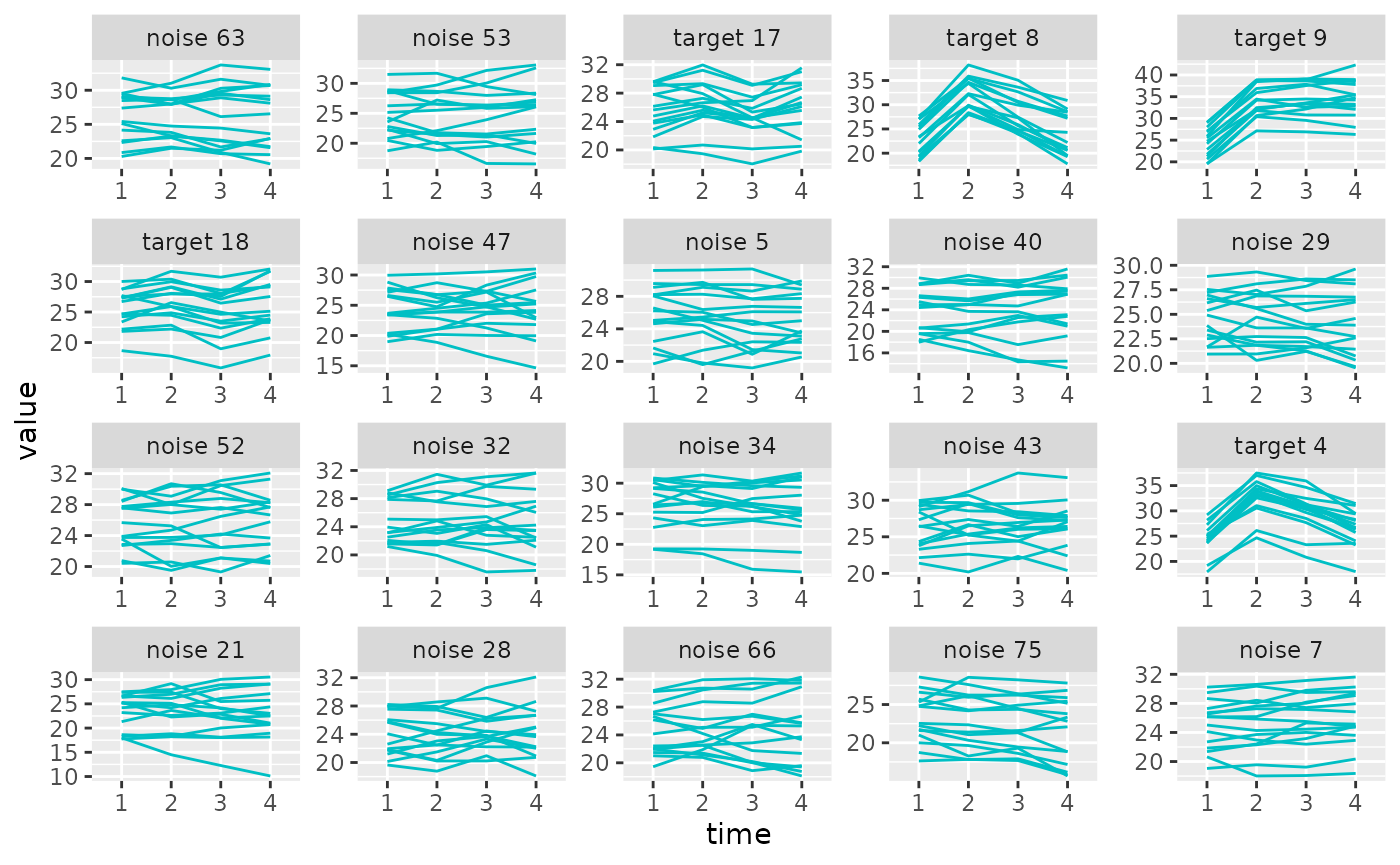

`prolong()` Function

Now that we have loaded our x array and y matrix, we can fit a lasso + laplacian and a group lasso + laplacian model. To fit the (non-group) lasso + laplacian model, we can specify groups = FALSE. If we don’t specify any of the model hyperparameters they will be automatically found.

promod_ll <- prolong(sim_metabs, sim_outcome, groups = FALSE)
#> No groups supplied or suggested, ordinary lasso will be used instead of group lasso
#> lambda2 and/or lambdar missing, optimizing over both
#> lambda2 = 0.275218954166098
#> lambdar = 0.017256334268004

Now that we have the results, we can quickly and easily visualize the selected variables with plot_trajectories().

plot_trajectories(sim_metabs, promod_ll)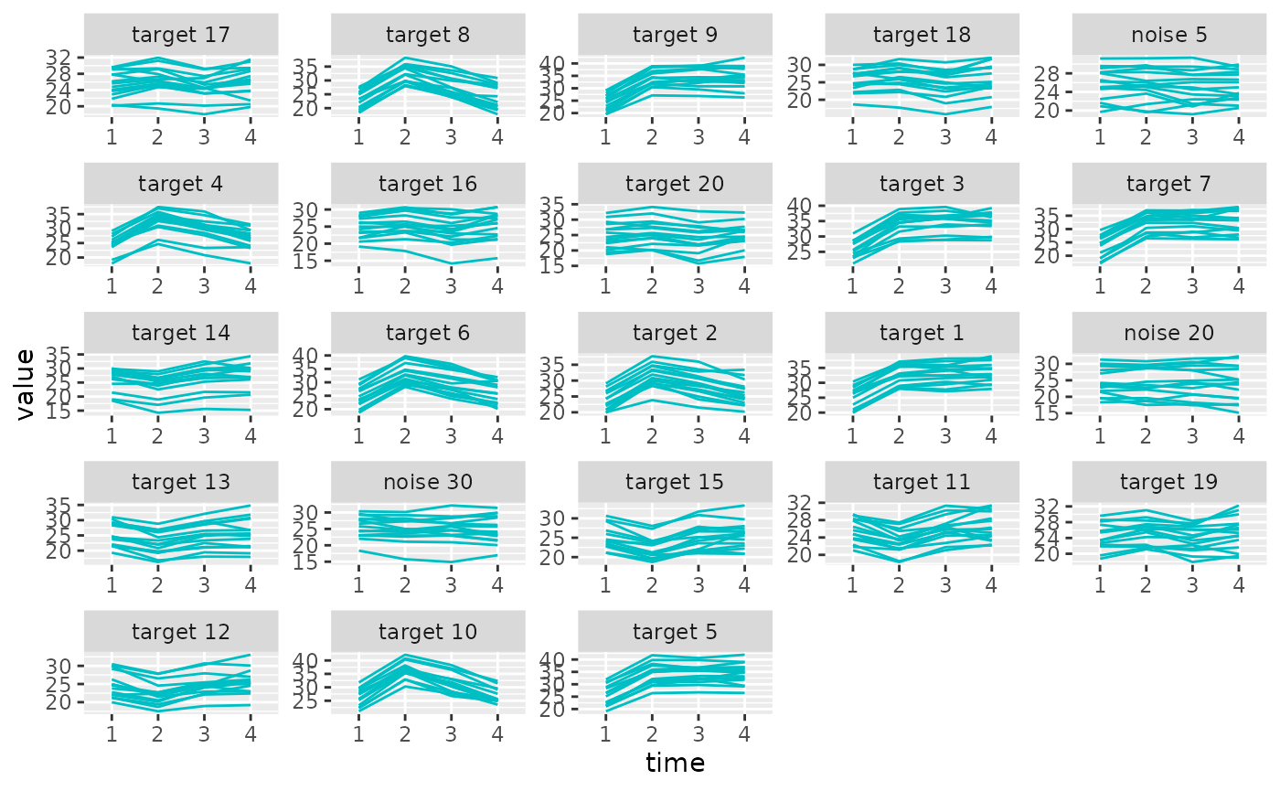

Let’s repeat the process but with the group lasso + laplacian model. The default is to automatically create 1 group for each of the \(p\) variables, with the different time point observations as replications within that group.

promod_gll <- prolong(sim_metabs, sim_outcome)
#> lambda2 and/or lambdar missing, optimizing over both
#> lambda2 = 0.275218954166098
#> lambdar = 0.017256334268004

plot_trajectories(sim_metabs, promod_gll)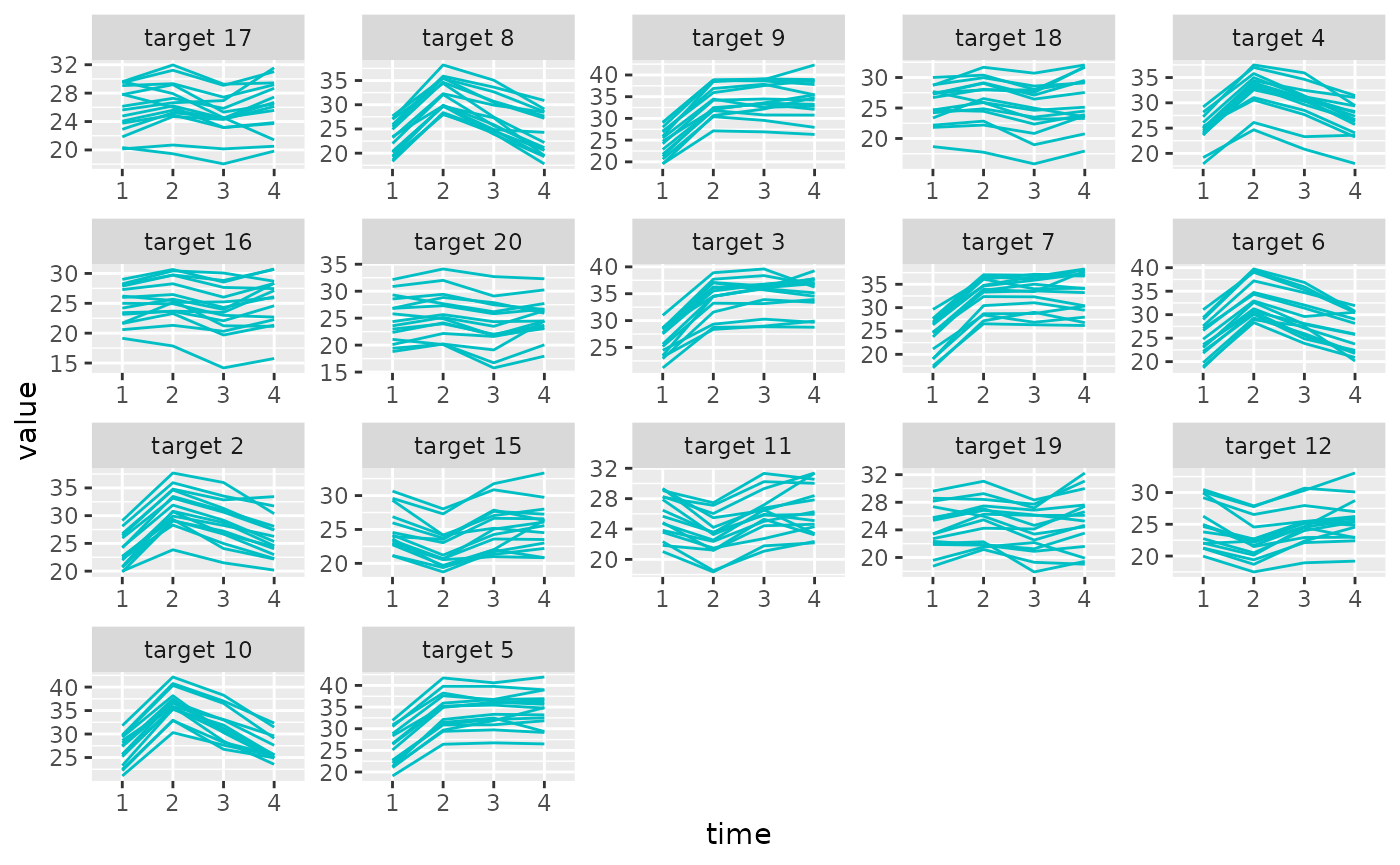

Correlation Plots

`delta_heatmap()` Function

The delta_heatmap() function takes the \(n\times p \times t\) array of variables and produces a heatmap of the delta-scale absolute correlations to visualize By default, delta_heatmap() will open a window to display an interactive Shiny app with the option to view a selected subsection of the heatmap.

delta_heatmap(sim_metabs)

If interactive = FALSE, then a static heatmap will instead be produced. We can also change the time points whose difference we take before computing the absolute correlation matrix.

delta_heatmap(sim_metabs, timediff = "3-2", interactive = F)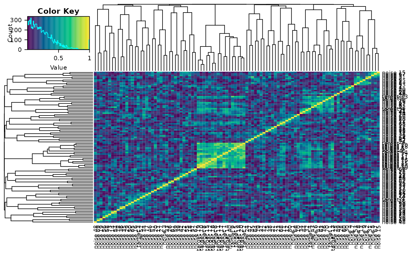

The delta_heatmap() function can also take in a prolong object, numeric list of columns, or column names to only show the heatmap for a selected subset of variables. These can be passed to arguments object = and selected = like with plot_trajectories

delta_heatmap(sim_metabs, timediff = '2-1', object = promod_gll, interactive = F)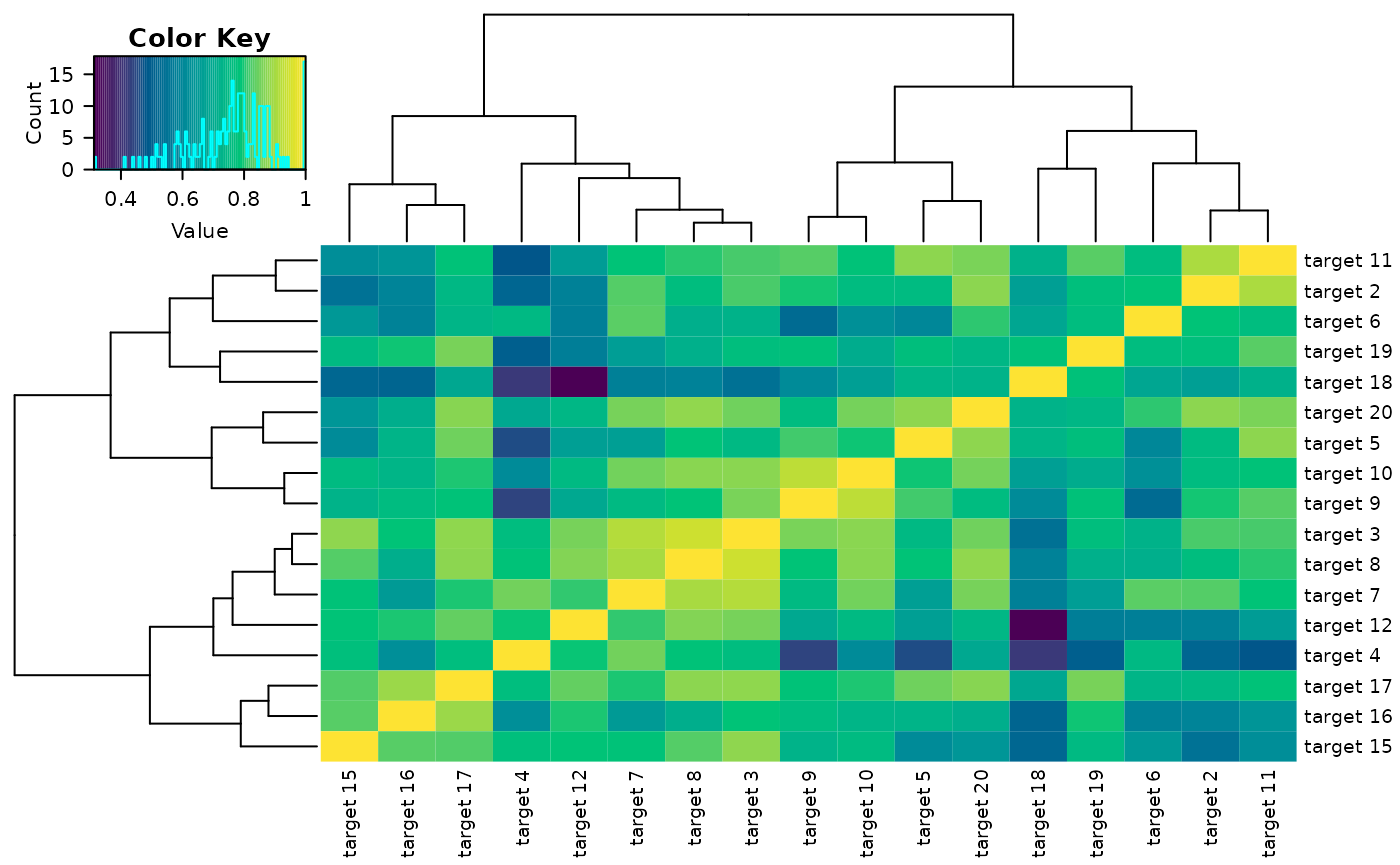

delta_heatmap(sim_metabs, timediff = '3-2', selected = promod_gll$selected, interactive = F)

Steve Broll